Evaluating Key Factors Influencing Scale Formation for Optimized Production in Gas-Lifted Oil Wells

Received 28 Feb, 2025

Accepted 22 Apr, 2025

Published 24 Apr, 2025

Background and Objective: Scale deposition in oil wells has been recognized to be a major operational problem as well as a major cause of formation damage, both in injection and producing wells. Scales contribute to equipment wear, corrosion, flow restrictions, and undesirable back pressures that cause a drastic decline in oil and gas production. This study presents a data-driven approach to investigate the effect of gas-lift injection rate on the scaling tendencies of oil wells. Materials and Methods: Mathematical models were used to obtain insight into the temperature and pressure profiles of gas-lifted wells as a function of gas injection rates, while the feed-forward neural network was used to develop a classification model to predict the status of the well regarding scale deposition. Univariate histogram/density distribution plots for the different variables to show how each variable influences scale precipitation, while pair plots that show the bivariate relationship between variables in the dataset and their influence on scale formation were also developed. A single-factor ANOVA was performed at a significance level of 0.05. Results: The classification model developed in this study accurately predicted the status of over 98% of the test wells, of which 37 wells were predicted to deposit scales and 68 not to deposit scales. The model only faltered in not adequately predicting two wells of their actual status. The accuracy, precision, sensitivity, and specificity of this model are 0.9813, 0.9855, 0.9855, and 0.9855, respectively. Conclusions: This model can provide benefits in investigating the scaling potential of gas-lifted wells compared to empirical models that apply simplifying assumptions with a high degree of accuracy.

INTRODUCTION

Oil production from depleted reservoirs is associated with very low drawdown that often results to a corresponding low oil flow rate. Depleted reservoirs lack sufficient energy to produce fluids into the wellbore and transport the same to the surface without an artificial lift system^1,2. The primary purpose of an artificial lift system is to lower the bottomhole flowing pressure and provide the lift energy necessary to transport the oil from the bottom of the well to the surface^3-5. Artificial lift systems designed for this purpose are broadly classified into two groups: The gas-lift system and the pumps.

Gas-lifting is a form of artificial lift method where compressed natural gas is injected via the gas-lift mandrels in the tubing-casting annulus to lower the viscosity of the crude in the tubing^6,7. The gas then mixes up and aerates the oil within the tubing, which lightens the fluid column that enhancing productivity through the reduction of viscosity and pressure losses⁸. This aeration process drastically reduces the hydrostatic pressure of the fluid in the tubing⁹. Gas-lifting can be done continuously or intermittently, depending on the case and severity of the problem. Irrespective of the lifting method deployed, gas lifting decreases the flowing bottomhole pressure, which consequently results to an increase in the pressure differential across the sand face and the in-situ reservoir pressure, the major driver of reservoir deliverability^10,11.

To plan for gas-lifting requires the assurance of lift gas in a field or adjacent fields to optimize the gas-lifting process. Unfortunately, due to competing projects, an increase in the demand for gas lift and other operating constraints can impose a limitation on the optimal recovery from gas-lifted wells. Assuming the only operating constraint to be the availability of gas lift in a field, the available gas lift must be optimally allocated among all gas-lifted wells to maximize oil production. Even where there is an unlimited available gas for gas-lifting, it is important to optimize the injection rate and take into consideration the gas utilization factor to maximize production from each gas-lifted well. Thus, the optimal allocation of available gas and the application of the optimal injection rate in gas-lifted wells to maximize productivity in a field is what could be termed the gas-lift optimization problem¹². Considering other operating conditions peculiar to a field and wellbore will generally result to a broader problem definition. Operating a gas-lift under too low or too high gas-lift injection rates has some disadvantages. If the gas lift injection rate is too low, the full lift potential of the gas-lift system would not be achieved, resulting in an inefficient operation⁸. Also, if the gas lift injection rate is too high, pressure surges induced by the gas lift in production facilities may be so high that they can lead to other operational problems; needless investments in compression, and other process equipment not necessary, and losses could be incurred⁸. In essence, gas lift design optimization seeks to initiate a cost-effective gas lift program by deciding the number of gas lift valves required, their depth, their respective operating pressures, the compressor discharge, and obviously, materials and equipment specification that will result in an optimum oil recovery at the lowest possible cost⁸.

The distribution of liquid saturation in hydrocarbon reservoirs makes it nearly impossible to produce hydrocarbons from these reservoirs without also producing some amount of water. As this produced water moves from the reservoir into the wellbore and up the production tubing, the pressure and temperature decrease. This decrease in pressure and temperature in the tubing has the potential to change the solubility of the salts originally dissolved in the formation water^13,14. Depending on the amount of water produced as well as the particular salts present in the formation water and its concentration, precipitation of salt minerals (scales) could occur around perforations, casing, along tubing, and even in surface equipment¹⁵. Scale is a mineral deposit that forms through a chemical reaction on downhole and surface facilities due to changes in temperature, pressure, and composition of an oil-water solution during production¹⁶.

When ion activities in a solution exceed their saturation limits due to changes in operational conditions, scale precipitation or crystallization could occur; and when these operational conditions degenerate further, the solution could become supersaturated, which could lead to scale deposition¹⁷. Thus, supersaturation of dissolved materials in solution is the main factor contributing to scale formation, when their concentrations exceed their equilibrium concentration in solution¹⁵. The degree of supersaturation, also known as the scaling index, determines the intensity of the precipitation reaction. A higher scaling index implies a greater likelihood of salt precipitation¹⁸. In addition to supersaturation conditions, particle nucleation and particle growth kinetics also play significant roles in determining the severity of scaling¹⁹.

Scaling during oil and gas production could be induced or self-scaling of mineral water. Generally, changes in operational conditions, such as a decline in pressure, temperature, changes in pH, and the mixing of incompatible waters from the formation or injection wells with other minerals, could trigger the precipitation and subsequent deposition of scales¹⁵. The injection of compressed gas during gas-lifting in itself can also cause changes in pressure, temperature, and composition of the in-situ fluid; this could also cause scaling²⁰. If the temperature or pressure of the well fluids deviates from the equilibrium values for the amount of dissolved minerals in the produced water accompanying the oil, it leads to the formation of inorganic scales. Scale precipitation in surface and subsurface oil and gas production facilities is a major operational problem and can cause damage to injection or producing wells. Scale deposition in oilfields leads to various technical and operational complications, and the severity varies in different production systems such as blockages in perforations, pipe obstructions, equipment damage, equipment wear, and corrosion, resulting in significant economic losses due to flow restrictions, decreased production rates, and operational downtime^21-26. Operational downtime could come from re-perforation, frequent replacement of down-hole equipment, re-perforation of scaling-producing intervals, reaming and re-drilling of plugged oil wells, stimulation of plugged oil-bearing formations, and various other remedial work-over operations²⁴.

Although gas-lift is an established technology for improving the performance of oil wells²⁷, injecting excess gas will either increase the bottomhole pressure which will lead to the decline in the liquid production rate²⁸ or alter the temperature and pressure of the well, that may result to the precipitation of inorganic scales²⁹; while injecting too small amount of gas will result to inefficient operation since the full lift potential of the gas is not utilized.

Dyer and Graham¹³ conducted a study on the impact of temperature and pressure on oilfield scale formation and observed that as pressure increased, the scaling tendency of carbonate and sulphate scaling brine decreased. Conversely, as the temperature increased, the scaling tendency of carbonate scaling brine increased while that of high sulphate scaling brine decreased. From this study, it could be inferred that temperature has a significant effect on scaling tendency compared to pressure. However, the study did not focus on how these changes in pressure and temperature can be induced or the extent to which they can vary due to operational factors.

In gas-lifted wells, the most commonly used technique for estimating the oil production rate is the Nodal analysis method. However, this method can be time-consuming and slow¹⁵. This slowness can be problematic in contemporary studies, such as closed-loop control of wells, where real-time optimization is desired. By the time the optimization process is completed using the traditional Nodal analysis method, the input parameters may have already changed. One factor contributing to the slowness of Nodal analysis is the estimation of temperature profiles in wells. Existing techniques like heat balance calculations are accurate but slow, while linear profile assumptions are faster but less accurate and not commonly used.

To address this issue, Mahdiani and Khamehchi¹⁵ proposed a combination model that integrates heat balance and linear temperature profile estimation methods. This approach offers a threefold increase in speed compared to traditional heat balance calculations while maintaining accuracy comparable to heat balance calculations. This new approach enables faster nodal analysis without sacrificing accuracy, making it more suitable for optimization purposes. Hasan and Kabir³⁰ introduced a technique for estimating the fluid temperature profile in gas-lifted wells using a mechanistic model. They emphasized the importance of understanding the temperature and pressure variations at the gas injection point and downstream for efficient gas-lift optimization. Assuming a linear temperature profile for the annular fluid had been a common practice, but a more holistic method of using a mechanistic model to account for the well depth and production time regardless of wellbore deviation angle was developed by Hasan and Kabir³⁰.

Several methods exist for predicting the formation of scale in oil and gas-producing facilities. Oddo and Tompson³¹ developed a simplified model for calculating the saturation index of CaCO₃ at high temperatures and pressures in brine solution using field parameters by changing the chemical equilibria of solutions of interest. Oddo and Tompson³² also observed that predicting scaling potentials could be difficult, developed different saturation indices and computer algorithms to predict if, when, and where scaling would occur in oil and gas production systems for barium, calcium, strontium, and magnesium sulphate scales. Hamid et al.³³ developed an empirical model using AI to predict scale growth rate at inflow control valves. Al-Hajri et al.²¹ developed a data-driven methodology that integrates production surveillance, chemistry, machine learning, and probabilistic theory to predict CaCO₃ scale formation in oil wells. Bahadori³⁴ developed a simple predictive tool to estimate the potential precipitation of CaCO₃ scale formation in saline aquifers used for CO₂ sequestration. Haarberg et al.³⁵ developed an equilibrium model for predicting the solubility products of scale-forming minerals in reservoir and production equipment during oil recovery. Most of these models predicted scale formation potential using either thermodynamics or the solubility index of scale-forming products during the production or injection of incompatible water. None investigated or predicted the tendencies of the factors that could promote scale formation during gas-lifting, even though some studies have investigated the prediction of tubing pressure distribution of gas-lifted wells³⁶. In this study, a machine learning classification model was developed to predict the occurrence of scale and also determine the key variables that could promote and strongly influence the deposition of scale during gas-lifting operations.

MATERIALS AND METHODS

Study area: This study was carried out using data obtained from 535 gas-lifted wells in the Niger Delta of Nigeria. The dataset included measurements of temperature, pressure, and various ion concentrations of the formation fluids. It targeted mainly gas-lifted wells. It was a research project that was conducted between March, 2022 and February, 2023 at the Department of Petroleum and Gas Engineering, University of Port Harcourt, Port Harcourt, Rivers State, Nigeria.

Mechanical modelling: The mechanistic model using the energy balance technique proposed by Hasan and Kabir³⁰ was adopted in this study to determine the temperature profiles of the tubing fluids as well as the temperature profile of the injected gas in the tubing-casing annulus of a well operating under gas-lift; while Kabir and Hasan³⁷ model was used to predict the pressure profile of gas-lifted wells and investigate the pressure variation within the tubing as a function of gas injection rate. Taitel et al.³⁸ was used to identify the flow regime transition from bubbly flow to slug flow, which is based on the gas void fraction within the tubing. The friction factor was determined using the explicit relationship by Chen³⁹ while the Reynolds’ number was estimated using the density and viscosity of the liquid phase, since the liquid is the continuous phase. A feed-forward neural network machine learning algorithm was then used to develop a classification model to predict the status of the well it will deposit scale or not.

Data presentation and analysis: To develop a reliable predictive model, the applicability and accuracy are directly associated with the validity of the dataset used for its development. Careful study on the mechanism of scale deposition shows that the main influencing variables that will be required as inputs into the machine learning model are^40,41,25:

	•	Temperature
	•	Pressure
	•	CO2 mole fraction
	•	pH and
	•	Ca2+, HCO3 , and CO32 concentrations

In developing the classification model, the state of the well as regards scale or not to scale was taken as the target. About 535 data points containing the above input variables were collected and properly pre-processed to minimize training errors. The basic techniques used for the pre-processing were noise reduction, handling of missing data points, and normalization.

Understanding the relationship between quantitative variables in a dataset is a necessary step in exploratory data analysis and is aimed at discovering patterns within the dataset that can be utilized for future prediction purposes. The collected field data were analyzed using different univariate and multivariate graphical formulations by looking into their statistical distributions in the form of histograms, scatter plots, and line plots

RESULTS AND DISCUSSION

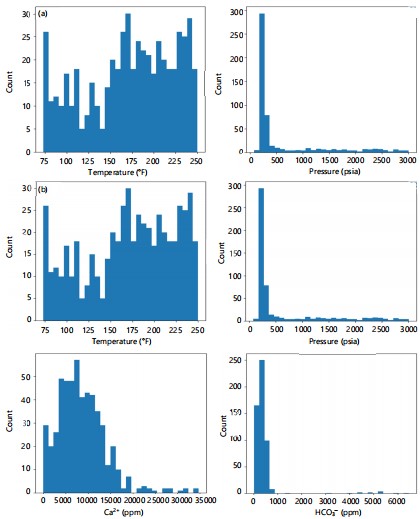
Table 1 shows the statistical description of the dataset obtained for scale appearance in oil wells as a function of some key parameters. It gives insight into the numeric distribution of the different parameters outlined for the study, including their minimum, maximum, mean, standard deviation values, as well as their first, second, and third quartiles as marked by the 25, 50, and 75% values, respectively. For example, as shown in Table 1, the temperature in the datasets ranged between 73 and 250°F, while the 1st, 2nd, and 3rd quartile values are 133, 177, and 214.5°F , respectively. The average of the 535 data points for temperature is 172.097°F and the standard deviation is 50.938°F. Similarly, the pressure datasets ranged between 82 and 3006 psia, while the 1st, 2nd, and 3rd quartile values are 235, 271, and 576.5 psia, respectively. The mean and standard deviation for the range of data sets is 633.954 and 732.942 psia. These trends were checked across other parameters that could influence scale precipitation and how they vary in the range of datasets considered in this study.

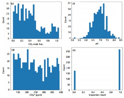
Figure 1 shows the univariate histogram/density distribution plots for the different variables that influence scale precipitation. Each peak indicates the density of values of a parameter in the datasets that fall within the range of values of a given parameter. For instance, values of temperature around 172°F has a mode of 30 as shown in Fig. 1a, while Fig. 1b shows that pressure of 250 psia has a mode of 290. The density distribution for other parameters is shown in Fig. 1(c-h), respectively.

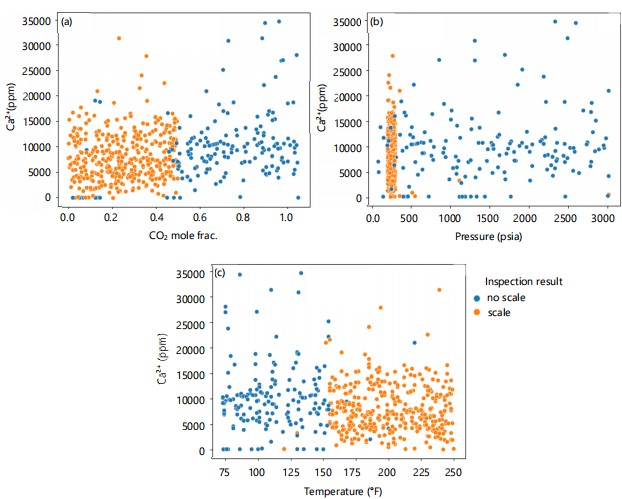
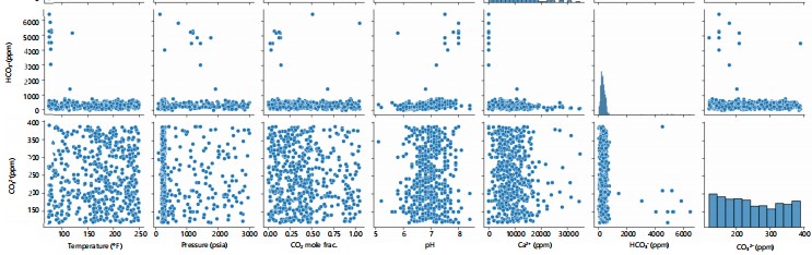
Investigations were made specifically to ascertain how changes in Ca²⁺ and CO₂ mole fractions, Ca²⁺ and temperature, as well as Ca²⁺ and pressure, affect scale deposition in wells using scatter plots as shown in Fig. 2a-c, respectively. From Fig. 2a, it can be seen that scale deposition is typically associated with wells producing water at lower CO₂ mole fractions. Figure 2b shows that scales also tend to precipitate at lower pressure, while Fig. 2c shows that higher temperatures facilitate the precipitation of scales, all for a given Ca²⁺ concentration. From the plots, it can also be seen that while the deposition of scale was noticed over a wide range of values for both the temperature and CO₂ mole fractions, the range of pressure over which scale deposited is within a narrow margin of 200-300 psia.

Table 1:

Statistical description of the dataset for scale appearance

	Temperature (°F)	Pressure (pisa)	CO2 mole frac.	pH	Ca2+ (ppm)	HCO3– (ppm)	CO3– (ppm)	Inspection result
Count	535.000000	535.000000	535.000000	535.000000	535.000000	535.000000	535.000000	535.000000
Mean	172.097196	633.95411	0.392932	6.930467	8666.1108	432.67365	245.9028	0.678505
Std	50.938062	732.94207	0.282606	0.474427	5474.5056	709.23719	80.898546	0.467488
Min	73.000000	82.000000	0.000057	5.100000	16.000000	26.000000	120.000000	0.000000
25%	133.000000	235.000000	0.169369	6.600000	4870.000000	216.000000	179.500000	0.000000
50%	177.000000	271.000000	0.341771	6.900000	7850.000000	317.000000	237.000000	1.000000
75%	214.500000	576.500000	0.548333	7.2.000000	11500.000000	442.000000	321.000000	1.000000
Max	250.000000	3006.000000	1.050000	8.4.000000	34700.000000	6466.000000	390.000000	1.000000

Fig. 1(a-f): Univariate histogram/density distribution plots for the different variables affecting scale appearance, (a) Temperature, (b) Pressure, (c) Ca2+, (d) HCO3–, (e) CO2 mole frac., (f) pH, (g) CO3 2– and (h) Inspection result

Each peak indicates the number of data points that fall within a given range of values

Fig. 2(a-c): Investigating the impact of different variables on scale deposition at a givenCa2+ concentration (a) Showing low mole fraction of CO2 and low concentration of Ca2+ promotes scale deposition, (b) Shows pressures in a narrow margin below 400 psia, and moderate concentration (below 200000 ppm) of Ca2+ promotes scaledeposition and (c) Showing high temperature (>150°F) and concentration of Ca2+ below 15,000 ppm significantly promote scale formation, respectively

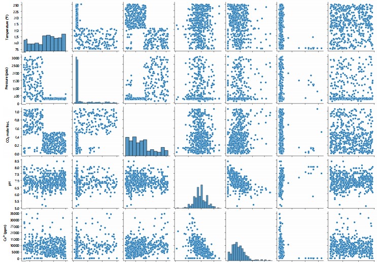
The pair plots showing bivariate relationships between variables in the dataset are shown in Fig. 3. These plots explain the numeric distribution and relationships between pairs of the variables in the dataset, like the temperature vs pressure, pressure vs CO₂ mole fraction, etc. For example, the temperature vs pressure bivariate plot in row 1, column 2 of Fig. 3, shows that most of the wells with temperature above 150°F had their pressure lower than 300 psia, while wells at lower temperatures exhibited much higher pressures. This indicates that extra precautions must be taken during the gas-lift operation in order not to increase the pressure over a certain range but to decrease the temperature well enough to minimize scale formation. The identity plots (e,g temperature vs temperature) are shown in histograms while the bivariate plots are in scatter diagrams. The identity plots are like Fig 1, which shows the range of distribution of each parameter value, while the scatter diagrams show the relationship among the variables investigated that could promote scale formation.

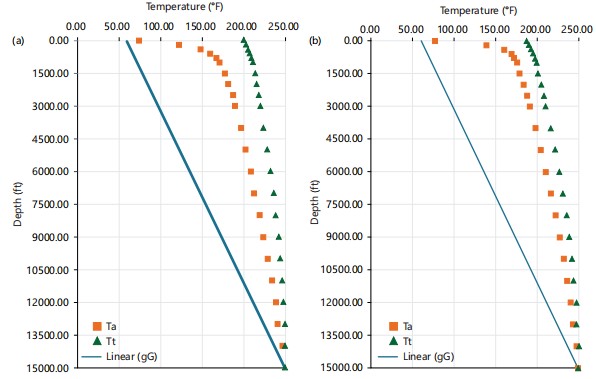
The Hasan and Kabir³⁰ model was used to investigate temperature variation of the fluid in the tubing caused by the injected gas, which leads to changes in the overall heat transfer coefficient. It was observed that the fluid temperature remained high in the entire length of the tubing if the oil production rate is kept reasonably high and the lift gas is injected at a rate that keeps the mass of the gas in the tubing annulus which reduces the overall heat transfer coefficient, thereby permitting the produced fluid mixture to retain most of its high entering enthalpy^42,43. Figure 3 shows an illustration of the effect of gas injection rate on the temperature profile of the well.

Fig. 3: Pair plot showing the bivaria te relationship between variables in the dataset about 10% of the total mass of the fluids. The high tubing fluid temperature was caused by the gas in the

From Fig. 4a and b, it can be seen that an increase in gas injection rate resulted in a slight decrease in the temperature of the tubing fluids measured at the same depth and oil flow rate due to the cooling from the expansion of the injected gas^44,45. The extent to which the temperature decreases depends on some factors, such as the overall heat transfer coefficient between the formation and the annular gas and the overall heat transfer coefficient between the tubing fluid and the annular gas^20,46.

However, owing to the low overall heat transfer coefficient between the tubing fluid and the annular gas which maintains the temperature of the tubing fluid fairly high throughout the length of the string^15,47,48 (except for the area very close to the wellhead), it becomes pertinent for an operator to diligently monitor the changes in pressure and other well parameters which affects scale deposition in order to keep the well scale-safe.

Fig. 4(a-b): (a) Temperature profile for a gas-lifted well at 5% gas mass fraction in the tubing and (b) Temperature profile for a gas-lifted well at 10% gas mass fraction in the tubing

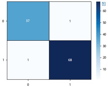
The machine learning model, when tested against the actual field data, was able to predict the state of the wells with an accuracy of over 98%. A visual representation of the performance of the classification model on the test dataset is presented in the form of a confusion matrix, as shown in the heatmaps of Fig. 5a and b. This matrix shows that out of the 107 data points in the test dataset, 37 of the wells predicted by the model to deposit scale deposited scales, and 68 wells that were predicted not to have scale deposition did not deposit scale. One of the wells predicted by the model to deposit scale did not, and scale was observed in one of the wells predicted not to deposit scale.

Aside from accuracy, other model evaluation metrics were used to evaluate the model performance, such as the precision score, the recall score, and the F1 score, each having its specific advantages over the other. A summary of these evaluation metrics for the classification models is given in Table 2. Which accurately predicted 37 wells to deposit scale and 68 wells not to deposit scale, while falsely predicting one well each to deposit scale and not to deposit scale.

Sensitivity analysis performed on the variables as shown in Table 3 to determine the impact of each variable on the outcome of the models’ prediction revealed that the temperature and the pressure were the most sensitive parameters for developing the classification model while the CO₂ mole fraction, pH, Ca²⁺, HCO₃^– and CO₃^2– contributed marginally to the final output of the model. This is in line with the study made by Dyer and Graham¹³ on the effect of temperature and pressure on oilfield scale formation.

While this study focused on investigating the tendency of scale appearance and deposition in gas-lifted wells, the main limitation lies in its narrow focus on carbonate scales, to the exclusion of other types of scales such as sulfates, halides, and silicates. This was a result of limited data on the other types of scales.

Future studies should consider expanding the scope to include other types of scales to provide a more general understanding of the complex dynamics involved in scale deposition.

Fig. 5: Confusion matrix showing the performance of the classification models

Table 2:

Different metrics used in model evaluation

Metric	Model performance
Accuracy score	0.9813
Precision score	0.9855
Recall score	0.9855
F1 score	0.9855

Table 3:

Sensitivity analysis scores for variables used in classification model showing the importance of each variable on the prediction of the model

Parameter	Significance
Temperature	0.1794839
Pressure	0.1124745
CO2 mole fraction	0.0450269
pH	0.0149293
Ca2+	0.0070929
HCO3–	0.0051459
CO32–	0.0030461

CONCLUSION

Gas-lifting is one of the well-known techniques for improving production from depleted reservoirs and, more especially, solution gas-driven reservoirs. However, gas-lifting has been identified as a potential cause of scale deposition in oil wells due to its effect on the temperature and pressure of the produced fluids. The effects of gas-lift operations on the temperature and pressure of the tubing fluids were studied, and a feed-forward neural network machine learning model was developed to predict scale formation in gas-lifted wells. Statistical metrics like the accuracy, precision, sensitivity, and specificity were used to evaluate the model when employed on a test dataset. The model was able to accurately predict the status of over 98% of the wells in the test dataset. Sensitivity analysis performed on the developed model indicated that the temperature and pressure were the two most sensitive parameters that determine the predicted values. Thus, since an increase in gas injection rate only caused a slight change in the temperature profile of the well, operators should therefore closely monitor the changes in the tubing pressure to keep the well within the scale-safe window while utilizing the optimal potential of the gas-lift system to enhance well productivity.

SIGNIFICANCE STATEMENT

One of the challenges encountered during gas-lifting is the formation of scale, which could occur from cooling effects from the injected gas when mixed with the in-situ fluid in the wellbore. The deposition of scale inhibits optimal production from oil wells and could also lead to the complete loss of production. In this study, the key parameters that promote the deposition of scale during gas-lifting were investigated, and it was observed that temperature changes pose the biggest threat, followed by pressure. Other variables have a minor influence on the deposition of scale. With this finding, it is important to ensure that excessive temperature variation is minimized during gas lifting to prevent the precipitation of mineral salts that could lead to scale formation.

REFERENCES

1. Hussein, A., 2023. Oil and Gas Production Operations and Production Fluids. In: Essentials of Flow Assurance Solids in Oil and Gas Operations: Understanding Fundamentals, Characterization, Prediction, Environmental Safety, and Management, Hussein, A. (Ed.), Elsevier Inc., Netherlands, ISBN: 978-0-323-99118-6, pp: 1-52.
2. Duru, U.I., O.I. Nwanwe, C.C. Nwanwe, A.O. Arinkoola and A.O. Chikwe, 2021. Evaluating lift systems for oil wells using integrated production modeling: A case study of a Niger Delta field. J. Pet. Eng. Technol., 11: 32-48.
3. Lea, J.F., 2007. Artificial Lift Selection. In: Production Operations Engineering, Lake, L.W. and J.D. Clegg (Eds.), Society of Petroleum Engineers, USA, ISBN: 978-1-55563-334-9.
4. Goswami, S. and T.S. Chouhan, 2015. Artificial lift to boost oil production. Int. J. Eng. Trends Technol., 26: 1-5.
5. Zeng, Z. and S. Cremaschi, 2018. Multistage stochastic models for shale gas artificial lift infrastructure planning. Comput. Aided Chem. Eng., 44: 1285-1290.
6. Allison, T.C., A. Singh and J. Thorp, 2019. Upstream Compression Applications. In: Compression Machinery for Oil and Gas, Brun, K. and R. Kurz (Eds.), Elsevier Inc., Netherlands, ISBN: 978-0-12-814683-5, pp: 375-385.
7. Janadeleh, M., R. Ghamarpoor, N.K. Abbood, S. Hosseini, H.N. Al-Saedi and A.Z. Hezave, 2024. Evaluation and selection of the best artificial lift method for optimal production using PIPESIM software. Heliyon, 10.
8. Abdalsadig, M.A.G.H., A. Nourian, G.G. Nasr and M. Babaie, 2016. Gas lift optimization to improve well performance. Int. J. Mech. Mechatron. Eng., 10: 512-520.
9. Takács, G., 2005. Gas Lift Manual. PennWell, Tulsa, USA, ISBN: 9780878148059, Pages: 478.
10. Lea, J.F., H.V. Nickens and M.R. Wells, 2008. Gas Lift. In: Gas Well Deliquification, Lea, J.F., H.V. Nickens and M.R. Wells (Eds.), Elsevier Inc., Netherlands, ISBN: 978-0-7506-8280-0, pp: 331-359.
11. Lea Jr., J.F. and L. Rowlan, 2019. Gas Lift. In: Gas Well Deliquification, Lea Jr., J.F. and L. Rowlan (Eds.), Elsevier Inc., Netherlands, ISBN: 978-0-12-815897-5, pp: 209-236.
12. Rashid, K., W. Bailey and B. Couët, 2012. A survey of methods for gas-lift optimization. Modell. Simul. Eng., 2012.
13. Dyer, S.J. and G.M. Graham, 2002. The effect of temperature and pressure on oilfield scale formation. J. Pet. Sci. Eng., 35: 95-107.
14. Abbasi, P., M. Madani, S. Abbasi and J. Moghadasi, 2022. Mixed salt precipitation and water evaporation during smart water alternative CO₂ injection in carbonate reservoirs. J. Pet. Sci. Eng., 208.
15. Mahdiani, M.R. and E. Khamehchi, 2016. A novel model for predicting the temperature profile in gas lift wells. Petroleum, 2: 408-414.
16. Cheng, J., D. Mao, M. Salamah and R. Horne, 2022. Scale buildup detection and characterization in production wells by deep learning methods. SPE Prod. Oper., 37: 616-631.
17. Hoang, T.A., 2022. Mechanisms of Scale Formation and Inhibition. In: Water-Formed Deposits: Fundamentals and Mitigation Strategies, Amjad, Z. and K.D. Demadis (Eds.), Elsevier Inc., Netherlands, ISBN: 978-0-12-822896-8, pp: 13-47.
18. Hashemi, S.H., Z. Besharati, F. Torabi and N. Pimentel, 2024. Thermodynamic prediction of scale formation in oil fields during water injection: Application of SPsim program through utilizing advanced visual basic excel tool. Processes, 12.
19. Li, J., M. Tang, Z. Ye, L. Chen and Y. Zhou, 2017. Scale formation and control in oil and gas fields: A review. J. Dispersion Sci. Technol., 38: 661-670.
20. van Thang Nguyen, M.K. Rogachev and A.N. Aleksandrov, 2020. A new approach to improving efficiency of gas-lift wells in the conditions of the formation of organic wax deposits in the dragon field. J. Pet. Explor. Prod. Technol., 10: 3663-3672.
21. Al-Hajri, N.M., A. Al-Ghamdi, Z. Tariq and M. Mahmoud, 2020. Scale-prediction/inhibition design using machine-learning techniques and probabilistic approach. SPE Prod. Oper., 35: 0987-1009.
22. Kamal, M.S., I. Hussein, M. Mahmoud, A.S. Sultan and M.A.S. Saad, 2018. Oilfield scale formation and chemical removal: A review. J. Pet. Sci. Eng., 171: 127-139.
23. Badr Bin Merdhah, A. and A.A.M. Yassin, 2007. Scale formation in oil reservoir during water injection at high-salinity formation water. J. Appl. Sci., 7: 3198-3207.
24. Olajire, A.A., 2015. A review of oilfield scale management technology for oil and gas production. J. Pet. Sci. Eng., 135: 723-737.
25. Rao, L.N., Y.M. Al Rawahi and S. Feroz, 2017. Studies on scale deposition in oil industries and their control. Int. J. Innovative Res. Sci. Technol., 3: 152-167.
26. Patel, J. and A. Nagar, 2022. Oil field scale in petroleum industry. Int. J. Innovative Res. Eng. Manage., 9: 288-293.
27. Yadua, A.U., K.A. Lawal, S.I. Eyitayo, O.M. Okoh, C.C. Obi and S. Matemilola, 2021. Performance of a gas-lifted oil production well at steady state. J. Pet. Explor. Prod. Technol., 11: 2805-2821.
28. Sukarno, P., D. Saepudin, S. Dewi, E. Soewono, K.A. Sidarto and A.Y. Gunawan, 2009. Optimization of gas injection allocation in a dual gas lift well system. J. Energy Res. Technol., 131.
29. Liu, K., X. Liu, H. Lou, L. Wu and R. Liao, 2024. Temperature and pressure prediction of offshore high CO₂-content associated gas lift and analysis of influencing factors. Geoenergy Sci. Eng., 241.
30. Hasan, A.R. and C.S. Kabir, 1996. A mechanistic model for computing fluid temperature profiles in gas-lift wells. SPE Prod. Facil., 11: 179-185.
31. Oddo, J.E. and M.B. Tomson, 1982. Simplified calculation of CACO₃ saturation at high temperatures and pressures in brine solutions. J. Pet. Technol., 34: 1583-1590.
32. Oddo, J.E. and M.B. Tomson, 1994. Why scale forms in the oil field and methods to predict it. SPE Prod. Facil., 9: 47-54.
33. Hamid, S., O. de Jesús, C. Jacinto, R. Izetti and H. Pinto et al., 2016. A practical method of predicting calcium carbonate scale formation in well completions. SPE Prod. Oper., 31: 1-11.
34. Bahadori, A., 2011. Estimation of potential precipitation from an equilibrated calcium carbonate aqueous phase using simple predictive tool. SPE Projects Facil. Constr., 6: 158-165.
35. Haarberg, T., I. Selm, D.B. Granbakken, T. Østvold, P. Read and T. Schmidt, 1992. Scale formation in reservoir and production equipment during oil recovery: An equilibrium model. SPE Prod. Eng., 7: 75-84.
36. Sami, N.A. and D.S. Ibrahim, 2021. Forecasting multiphase flowing bottom-hole pressure of vertical oil wells using three machine learning techniques. Pet. Res., 6: 417-422.
37. Kabir, C.S. and A.R. Hasan, 1990. Performance of a two-phase gas/liquid flow model in vertical wells. J. Pet. Sci. Eng., 4: 273-289.
38. Taitel, Y., D. Bornea and A.E. Dukler, 1980. Modelling flow pattern transitions for steady upward gas-liquid flow in vertical tubes. AIChE J., 26: 345-354.
39. Chen, N.H., 1979. An explicit equation for friction factor in pipe. Ind. Eng. Chem. Fundam., 18: 296-297.
40. Oliveira, D.F., R.S. Santos, A.S. Machado, A.S.S. Silva, M.J. Anjos and R.T. Lopes, 2019. Characterization of scale deposition in oil pipelines through X-ray Microfluorescence and X-ray microtomography. Appl. Radiat. Isot., 151: 247-255.
41. Hari, S., S. Krishna, M. Patel, P. Bhatia and R.K. Vij, 2022. Influence of wellhead pressure and water cut in the optimization of oil production from gas lifted wells. Pet. Res., 7: 253-262.
42. Pu, C., 2022. Prediction and analysis of annular pressure caused by temperature effect for HP/HT/HHS and water production gas wells in Sichuan Basin. J. Pet. Explor. Prod. Technol., 12: 507-517.
43. Oudeman, P. and M. Kerem, 2006. Transient behavior of annular pressure build-up in HP/HT wells. SPE Drill. Complet., 21: 234-241.
44. Han, G., H. Zhang, K. Ling, D. Wu and Z. Zhang, 2014. A transient two-phase fluid- and heat-flow model for gas-lift-assisted waxy-crude wells with periodical electric heating. J. Can. Pet. Technol., 53: 304-314.
45. Gao, K., Q. Zhao, X. Zhang, S. Shang and L. Guan et al., 2023. Temperature field study of offshore heavy oil wellbore with coiled tubing gas lift-assisted lifting. Geofluids, 2023.
46. Wiktorski, E., C. Cobbah, D. Sui and M. Khalifeh, 2019. Experimental study of temperature effects on wellbore material properties to enhance temperature profile modeling for production wells. J. Pet. Sci. Eng., 176: 689-701.
47. Mu, L., Q. Zhang, Q. Li and F. Zeng, 2018. A comparison of thermal models for temperature profiles in gas-lift wells. Energies, 11.
48. Guo, B. and J. Song, 2016. An improved model for predicting fluid temperature in deep wells. Math. Modell. Appl., 1: 20-25.